
This is part 2 of 2 of the MRD blog post. (Click here for part 1).
In this section, we will discuss how to overcome some of the most common challenges of MRD testing.
Overcoming the Challenges
In order to mitigate sequencing errors, methods using Molecular Barcodes (MBCs), Unique Molecular Identifiers (UMIs), etc. (which are essentially all the same) may be used, where each starting molecule is sequenced many times. The MBCs are then used to generate consensus sequences from sequences that were likely obtained from the same starting molecule. The assumption is that errors appear due to somewhat stochastic processes and that the consensus sequences will likely be correct. This requires many observations of the same starting molecule, so it will be recommended to generate 10-fold more sequences than there are molecules. Therefore, with 8,000 genomic equivalents, we might want to target a sequencing depth of 80,000. This is a reason why using 10-fold more input ccfDNA may not necessarily be a good thing (in addition to having to obtain a 10-fold larger liquid biopsy) since we may have to increase sequencing depth accordingly to 800,000, which could increase the cost of sequencing 10-fold, which could reduce the likelihood for payment and running the assay profitably.
The use of dual MBCs – as is the case in Agilent’s SureSelect XT HS2, Illumina’s TSO 500, Roche’s AVENIO, etc. assays – further allows consensus sequences to be derived from both starting DNA strands of a molecule. If a somatic mutation is present on the starting molecule, then both strands should support the presence of that mutation. If an apparent mutation is only observed on one strand – for example, due to cytosine deamination of the starting molecule – then there may not be any support for that mutation from the other strand.
However, the types of mutations that appear due to the assay and sequencing are not completely stochastic. Some types are much more common than others and, by sequencing many normal samples, one can get an idea of what types of mutations are less likely to appear than others. Cytosine deamination can occur through heating, and the first PCR step, where DNA is denatured and a thermostable polymerase is activated, often involves a several minute ~94 °C incubation. This can then lead to the formation of C>T variants (that may also be observed as G>A). However, these variants may have little support from the other DNA strand – except when they do. With a large enough panel – especially, when there are few replicates of starting molecules – there will probably be some C>T variants that make it through MBC-based error correction. Similarly, A>G (T>C) has been noisy in NGS data that I have looked at. Therefore, if we are going to detect variants based on 1 or 2 observations, then it can be helpful to avoid types of mutations that are noisier than others, which may have implications for managing noise that may need to be platform- and assay-specific.
The goal of an MRD monitoring assay is different from a ctDNA assay used for somatic mutation identification. In MRD monitoring, we are less concerned with detecting new somatic mutations than we are with detecting previously-identified mutations that are expected to be present in the tumor. Thus, the quality of all sequenced bases is less important than the quality of the bases where somatic mutations are believed to reside. So, while we may need to call existing somatic variants with few observations, we would not be attempting to call new somatic mutations.
At low tumor content, somatic variants become difficult to detect because they may not be present in the sample – or at a sufficient number of copies. A solution is to look for many somatic variants. However, a sample with a low Tumor Mutational Burden (TMB) of say 5 would only have around 10 in a 2 megabase ctDNA panel, which can cost several thousand dollars to run. Therefore, we may want to use patient-specific panels that only look for mutations that are found in the tumor of this patient. Whole Exome Sequencing (WES) can be used as a first step, if a regular tumor biopsy is available. A sample with a TMB of 5 would be expected to have around 150 variants in exons. With whole genome data, there may be 10,000 variants to choose from. With more variants to choose from, there are more opportunities to choose variants that can be detected with good sensitivity and specificity. Sensitivity is important since we want to be able to detect variants when they are present. Specificity is important since – if we are going to detect a variant with a single observation – we do not want to have a single observation of a variant that is not there.
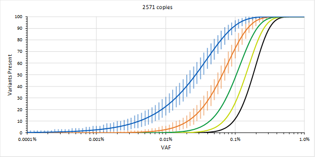
Figure 1. High sensitivity requires decisions made from few observations. Expected number of called somatic variants out of 100 for a given VAF and for different numbers of minimum observations required to call a variant in 30 ng of DNA (blue = 1, orange = 2, and others = 3 to 5 observations)
The sensitivity obtained by detecting variants with a single observation and only requiring one out of a 100 variants to be detected, per the FDA guidance, could allow the assay to be used for MRD defined at ~0.01 % VAF for selecting patients. On the other hand, if we need two observations before we are willing to call a variant, then the LOD increases by an order of magnitude. If we need more than one variant to be called, then the LOD increases further.
If we manage to increase the ccfDNA input, then this is expected to improve sensitivity; provided, that we increase sequencing depth accordingly. Additionally, we could also increase the number of variants we are looking for. However, as mentioned previously, a TMB of 5 corresponds to about 150 variants identified by WES and not all of those may be desirable (e.g., C>T); and, some patients may have tumors with significantly fewer identified mutations.
Validating Patient-Specific Assays
A regular ctDNA panel, provides many performance data points for the same locations in the genome, allowing for the tuning of the ctDNA assay and associated pipelines to work well for identifying somatic variants in those locations. However, patient-specific assays are different; and, validation may need to include the process of designing many different custom assays for somatic variants that are located all over the genome since each patient is different. This would be followed by assessments of the sensitivity and specificity of those custom assays to determine whether the approach meets end user requirements for MRD monitoring.
To enable such validation, the LGC SeraCare poster presented at AACR’s virtual session II titled “Reference materials for measurable residual disease (MRD) monitoring” (#1978) describes a new set of reference materials for MRD assays. The reference materials featured in this poster utilize germline SNP-matched cell lines for a tumor/normal workflow.
The tumor and normal components can be used for WES or other assays to identify somatic mutations in the tumor components; or, one can just obtain the WES data from SeraCare. Custom assays can then be designed to detect those somatic mutations and evaluate sensitivity and specificity; the poster describes a design of two different custom NGS MRD assays. Since the tumor components have a TMB in the 10-20 range (~300+ somatic mutations in exons) and are ~euploid, the reference materials can be formulated for LOD studies where the somatic mutations are present at defined frequencies.
Therefore, if we want to determine how well the MRD monitoring assay detects somatic variants at 0.01 % VAF or even at or below 0.001 % VAF, then these reference materials can be used. Interestingly, data in the poster shows that when variants are chosen well, MBCs may not be necessary for evaluating somatic variants at 0.1 % VAF (at least on an Illumina MiSeq with 8 samples per flow cell). However, 0.1 % VAF is only the starting point for MRD monitoring, and limited error correction may allow for the detection of somatic variants at 0.01 % VAF when targeting only about 20 somatic mutations.
One third of the mutations were used to assess sensitivity in a given tumor component, while the rest of the mutations were used to assess specificity since they were only expected in one of the other two tumor components. By designing a single custom assay to evaluate MRD in two or more patients, the mutations that are not expected to be observed in a given patient may be used to evaluate the specificity when using 1 or 2 observations to call a somatic mutation. If there is more specific signal than noise, then there may still be MRD.
While 0.01 % VAF was close to the limit of detection with about 20 somatic mutations assayed per tumor (~0.02 % tumor content), we could increase that number to 100 somatic mutations for our custom assay to potentially improve the LOD – although, the assay may be more expensive to run due to the need for proportionally more sequencing. At the same time, the ~300+ somatic mutations in the exons of each tumor component could be used to design many custom assays and evaluate the ability of a given custom assay to have similar performance. If more somatic mutations are needed, then somatic mutations could be determined in introns as well, or reference materials derived from additional SNP-matched tumor/normal components could be used.
Conclusions
In conclusion, if we are going to design assays for MRD monitoring, then those assays will be different from conventional ctDNA assays. They may need to detect variants with fewer observations while maintaining specificity in order to have sufficient sensitivity. At the same time, they may need to be customized for the somatic mutations in a given patient, which means that the whole process from somatic mutation identification, through custom NGS panel design, through MRD monitoring may need to be validated. Luckily, there are now reference materials for this - Reference Materials for Measurable Residual Disease (MRD) Monitoring.
Designing Patient-Specific Assays
To model ideal assay performance, we can use Poisson and Binomial distributions in Excel. To determine the fraction of variants that will have at least count_at observations given a certain number of average observations (avg_obs), the following equation can be used:
=1-POISSON.DIST((count_at-1),avg_obs,TRUE)
For example, if we normally require 5 observations of a variant to call it as present and we expect a sample to contain about 8 detectable copies of variants, then we would use the following that predicts that we would call 90 % of such variants (we integrate the area of the Poisson distribution for 0 to 4 observations, then subtract that from the total area of 1 to obtain the area for 5 or more observations):
=1-POISSON.DIST((5-1),8,TRUE)
If there are only about 2 detectable copies of each variant, then we would only be able to call about 5 % of such variants. The number of detectable variants would be obtained by multiplying that by the number of variants we are looking for. So, the more variants we look for, the higher the likelihood of detecting at least some variants. However, looking for more somatic variants requires sequencing more. Additionally, looking for more somatic variants has the potential to increase the number of false positive variants.
The confidence interval for the number of variants we would call present can be obtained from the total number of variants (total_vars), the fraction of detectable variants (fraction), and the lower and upper bounds of the confidence interval (location; either 0.025 or 0.975 for a 95 % confidence interval):
=BINOM.INV(total_vars,fraction,location)
In the example above, if there are only about 2 detectable copies of each variant and we are looking for 100 variants, then we would expect to call between 1 and 10 variants 95 % of the time. Setting location to 0.05 would give us an idea of the LOD since 95 % of samples would have at least 2 out of 100 variants called present when there are an average of about 2 detectable copies of each variant. If those two called variants mean that the sample is MRD positive in our assay, then our LOD would be a sample that averages 2 detectable copies. For 30 ng, that would be an average VAF of 0.025 %. However, 100 % of input will probably not be analyzable and 30 % may be more typical. In that case, the average VAF would be just below 0.1 %.
However, we may want to get to 0.01 % or 0.001 % or even lower average VAFs. WES for a sample with a TMB of 5 will give us about 150 variants, but not all of those will be ideal. To get to those lower average VAFs, we need to get comfortable with calling variants at 1 or 2 observations.
